Sparse, Adaptive Hypernetworks
Many types of data in modern machine learning are highly structured: vector images, (knowledge) graphs, natural language, etc. Such data is usually best stored in sparse format: often using one-hot coding for the individual elements, and something akin to an adjacency matrix for the relations holding them together. Consequently, the transformations we want to learn for such instances are also highly sparse.
Consider, for instance the example of learning a graph-to-graph transformation for directed graphs. We will allow self-loops, but not multiple connections, so that each graph can be represented by a square, binary adjacency matrix. Let us also assume that we want to learn a simple graph transformation. The most straightforward approach would be to use a single, fully-connected layer from one adjacency matrix to another: \(y = Wx\) with \(x\) the input adjacency matrix, \(W\) the weight matrix, and \(y\) the output.
In this scenario, our input is likely very sparse: for large, natural graphs, most elements of the adjacency matrix are usually zero. Therefore, most elements of \(W\) should also be zero. Unfortunately, the structure of our data is not regular. When processing images, we know in advance that each instance will consist of a grid of pixels, and we can wire our network accordingly for the whole dataset. In our case, each instance contains a new structure, which is encoded in the input itself. We must therefore learn the sparse structure of our transformation adaptively.
In a naive implementation, this would still require a dense datastructure to store the weights \(W\). Even though the matrix we end up with will be sparse, we don’t know a priori if a particular weight will be zero or not for any given instance, so all zero weights must be stored explicitly. Assuming that the output of our transformation is as large as the input, the number of weights of our layer grows as the square of the size of the input. Since the size of the input is already the square of the number of nodes in the network, this is clearly an unfeasible approach for large graphs.
Non-adaptive sparse transformations
Our proposed solution is to represent \(W\) as a sparse matrix, even during training. Sparse matrix datastructures are nothing new: we simply store the index tuples \(I\) of the non-zero values of \(W\), together with their values \(V\) in a long list, and we assume that all other elements of \(W\) are zero. There are many efficient ways to perform matrix multiplications with sparse matrices stored this way, even on the GPU.
The trick to learning sparse matrices is to make \(I\) and \(V\) both parameters. That is, we learn not only the values of \(W\) through backpropagation, but also their indices. We simply create one k-by-2 integer matrix \(I\) for the indices (one index-tuple per row) and a length-k vector \(V\) for the values. And try to learn both \(I\) and \(V\). Unfortunately, gradient-based methods don’t work well for integer parameters. If we have an integer tuple at \((12, 13)\) that should be at \((13, 13)\), the gradient is not going to tell us that we’re close to a good solution. We need to represent the integer tuples in a continuous space, and translate them to integers to construct the weight matrix.
One option is to define a probability distribution over the index-tuples and to use stochastic nodes in the computation graph [1] to sample them, which is essentially like using reinforcement learning. This is usually very slow, and difficult to train. We take a different approach: instead of using stochastic nodes in a fixed computation graph, we create a non-stochastic computation graph, but wire it stochastically for every batch.
First, we extend the definition of each index tuple: for each tuple \(i\), we define a multivariate normal distribution with a 2D mean \(\mu_i\) and a single scalar variance parameter \(\sigma_i\). This is meant as a continuous distribution to represent uncertainty over the discrete index tuples (bear with me). The aim is that \(\sigma_i\) starts relatively large at the start of training, but slowly goes to zero, as \(\mu_i\) converges to an integer value.
To accomplish this, we sample integer tuples uniformly*. We then divide the value \(v_i\) over the sampled index tuples in proportion to the probability density each receives under \(N_{\mu,\sigma}\). This means that the integer tuples we sampled are detached from the computation graph. The backpropagation signal goes only through the values, but the values are computed using the parameters of the MVNs.
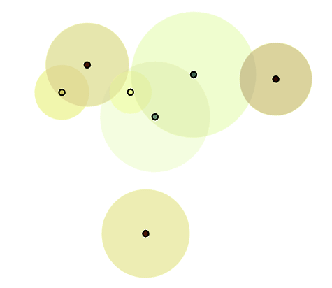
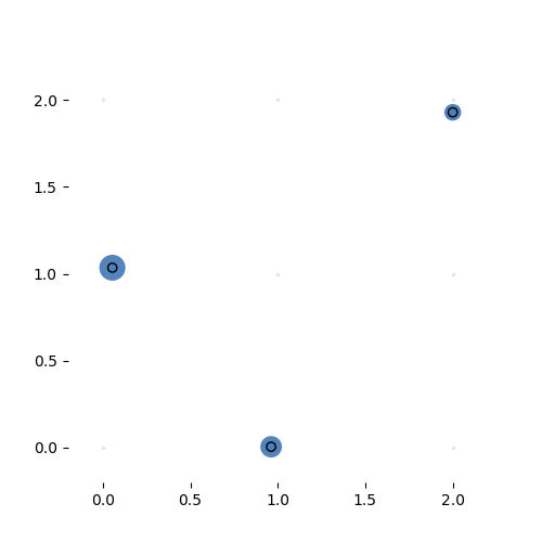
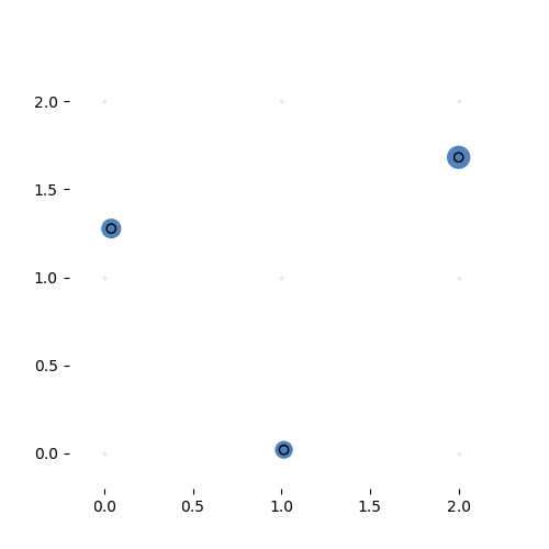
If that sounds confusing here’s what it looks like in action. The task is simple: learn the identity function from \({\mathbb R}^{32}\) to \({\mathbb R}^{32}\) (ie. learn the 32-by-32 identity matrix). We give the model exactly 32 MVNs to learn, and sample 68 integer tuples per instance, per MVN.
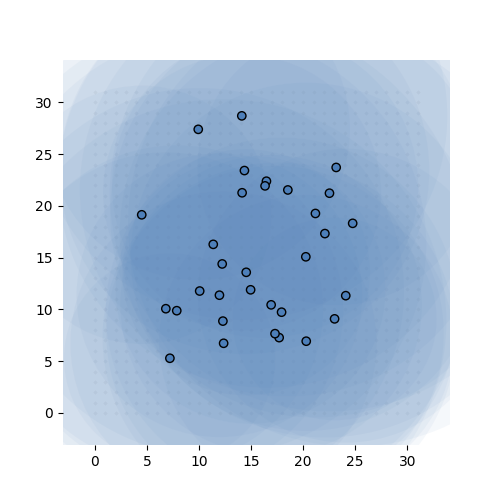
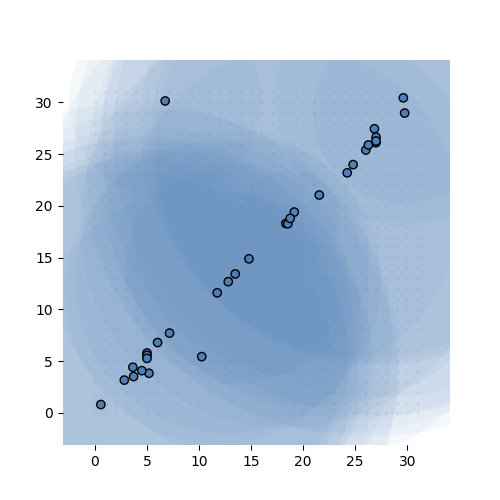
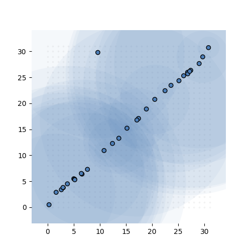
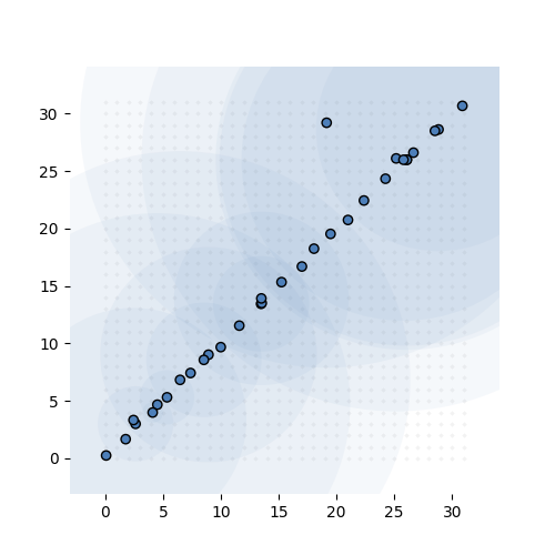
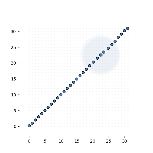
Learning the 32-by-32 identity matrix (after 0, 1k, 2k, 3k and 6k batches of 256 instances observed). Each dot represents the mean of one of the MVNs. The values are fixed to 1 for this experiment. The transparent circle represents the variance of the MVN.
Sparse, adaptive hypernetworks
This gives us an efficient way to learn highly sparse transformations, but they are not yet adaptive. The transformation is fixed. To make it adaptive, we use a hypernetwork to produce the index-tuple MVNs and the values.
This hypernetwork get a view of the input, possible downsampled, and produces the full parameter matrix for the sparse transformation through a series of deconvolutions.
Here it is learning a more complex variant of the identity task. The task is to reproduce the input vector, but sorted. This is a highly nonlinear transformation, but for certain partitions of the input space, the transformation is simply a permutation matrix. If the hypernetwork can learn to produce the right permutation matrix, we can solve this problem with one sparse, adaptive hyperlayer.
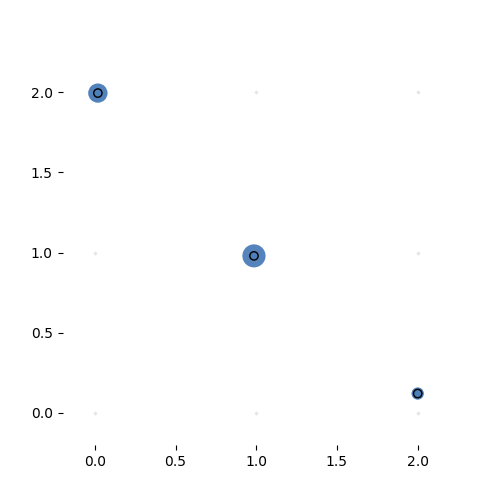
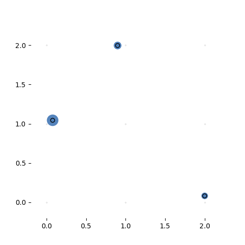
Learning the 3-by-3 sorting transformation. Iterations 7000, 7050, 7100 and 7150 (with a batch of 64 per iteration). Note that the source network is generating a new permutation matrix for each input.
Real tasks
Does it scale to real world tasks? Well that’s where I’m at now. So far, I have a two layer model that gets about 90 percent accuracy on MNIST. If you know MNIST, you’ll know that that’s not stellar. Still, the model is extremely sparse, and a simple convnet with similar tensor shapes on the hidden layers doesn’t do any better. I need to do some more experimenting with architectures to see what works (within the limit of available GPU memory).
I’m aiming to show the following:
- On small-sized image datasets (MNIST, CIFAR), I can achieve performance competitive with simple baselines.
- On high res images (e.g. COCO), the ASH model can function as a kind of attention mechanism. That is, the source network analyses a downsampled version of the image, and tells the ASH layer what to focus on.
- Using a Variational Autoencoder consisting of ASH layers, we can learn a basic generative model for small graphs.
The following tricks are crucial to scaling up:
- There’s no simple way to initialize the layer well. One option is to pretrain with an autoencoder, but that takes a while. Instead, I’ve found it useful to add a small reconstruction term for each layer to the loss (usually with a 0.01 multiplier). This helps to guide the network to useful representations while the for gradient from input to output is not yet informative.
- ConvNets may be sparse, but they still have quite a lot of non-zero elements when you represent them as a sparse matrix. In order to reach this scale, we need to sample a subset of the index tuples to train each batch. This seems to work if the subsample isn’t too small. It even improves performance if we subsample half the tuples. Work in progress.
- To truly mimic a ConvNet, we need a way to share parameters within a sparse layer (a single convolution can have as few as 9 parameters). We can’t use the trick we used earlier of multiplying out a single value proportionally over samples, because that would lead to soft-weight sharing (which doesn’t actually increase the simplicity of the network). We need something that forces the network to converge towards a fixed choice of, say, 15 source scalars for each non-zero value in \(W\). These 15 scalars can then also be learned through backprop. To really force a choice rather than a mix, we need to use stochastic nodes here. I have a working implementation, but the effects aren’t clear yet. Also work in progress.
- The variances of the MVNs describing the index tuples tend to go to zero a little too quickly. This means that even if one of the correct index tuples is sampled, the gradient is too small to be picked up. For now, a loss term punishing small gradients alleviates the issue. There may be a more elegant solution, like choosing a fat tailed distribution instead of an MVN.
Code and links
If you’re brave enough to dig into my galaxy of spaghetti code, you can find everything here. I can’t promise to answer questions or help out, but you’re free to ask (on github, twitter or email). The project is written in PyTorch, because it depends on dynamic graphs. Nowadays, we have eager mode, so a Tensorflow port is probably an option.
References
- [1] Schulman, John, et al. “Gradient estimation using stochastic computation graphs.” Advances in Neural Information Processing Systems. 2015.